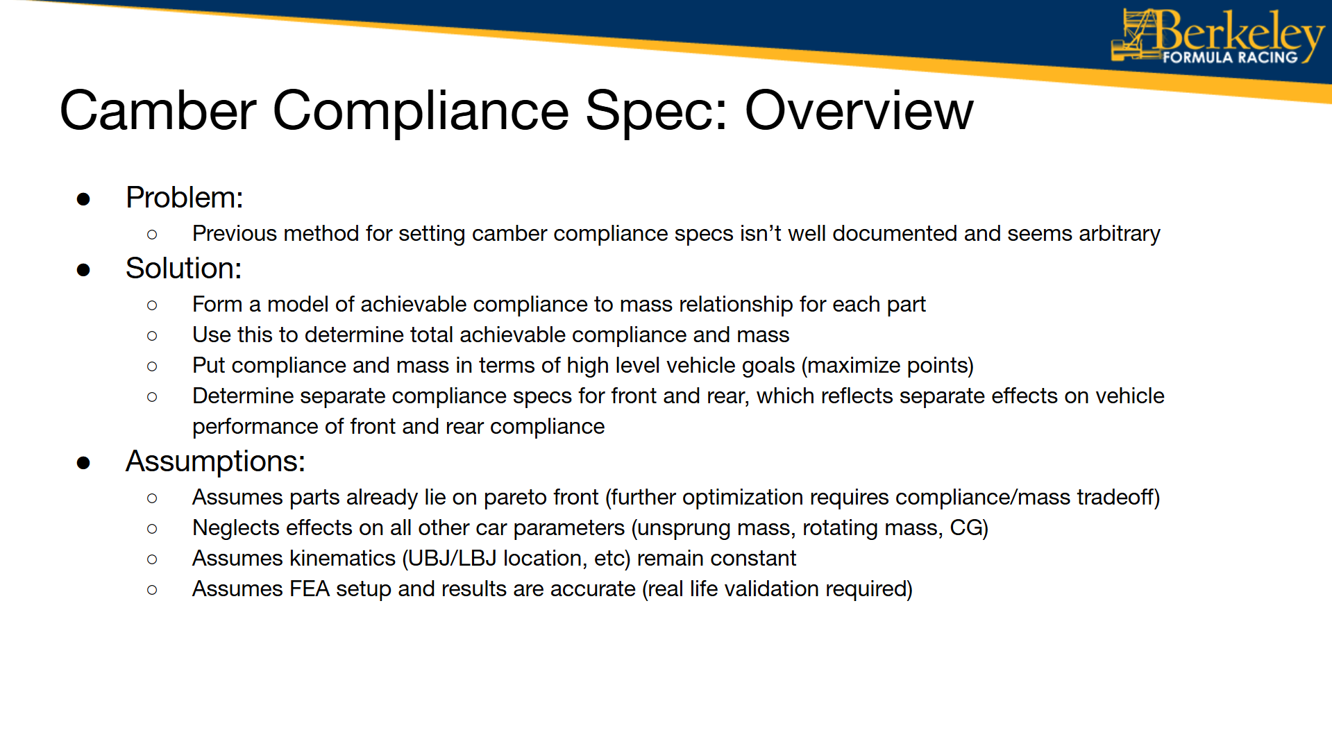
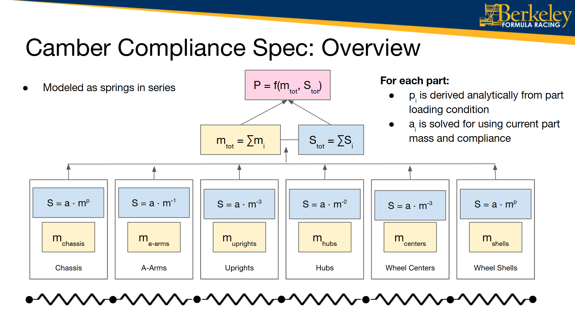
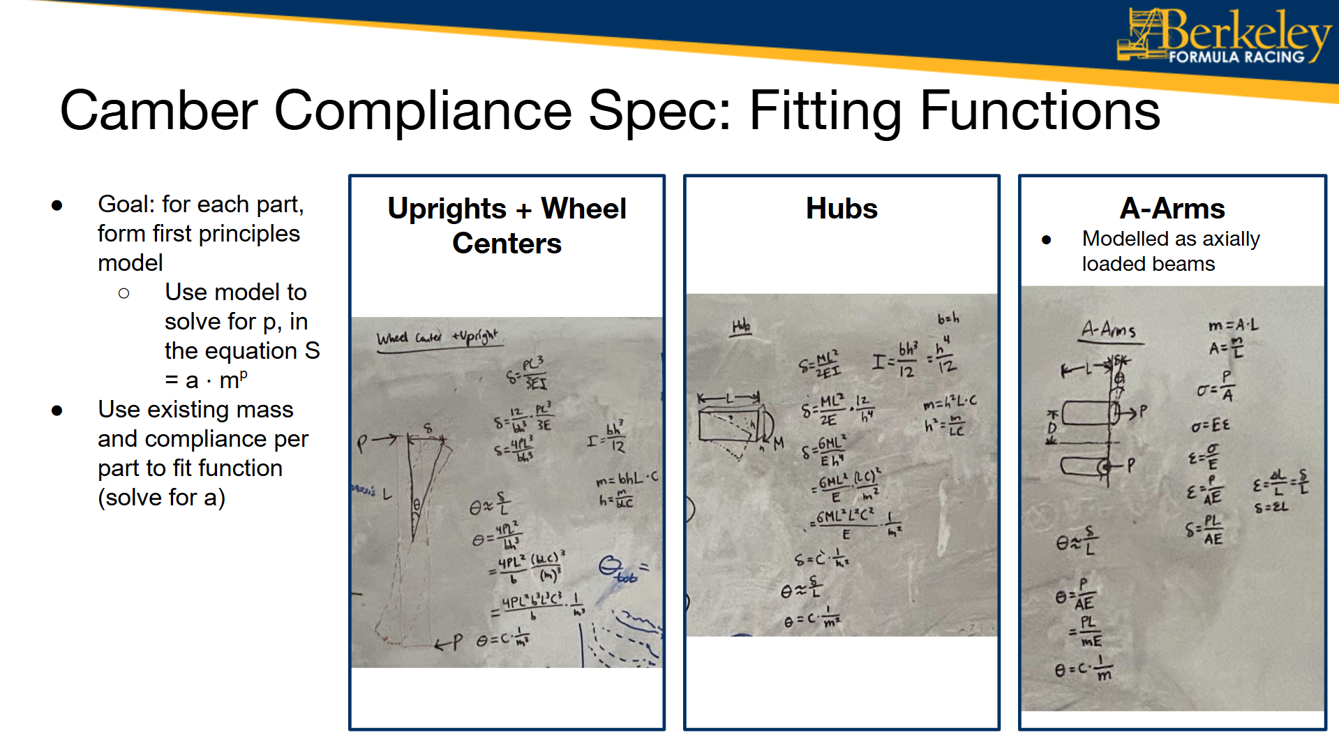
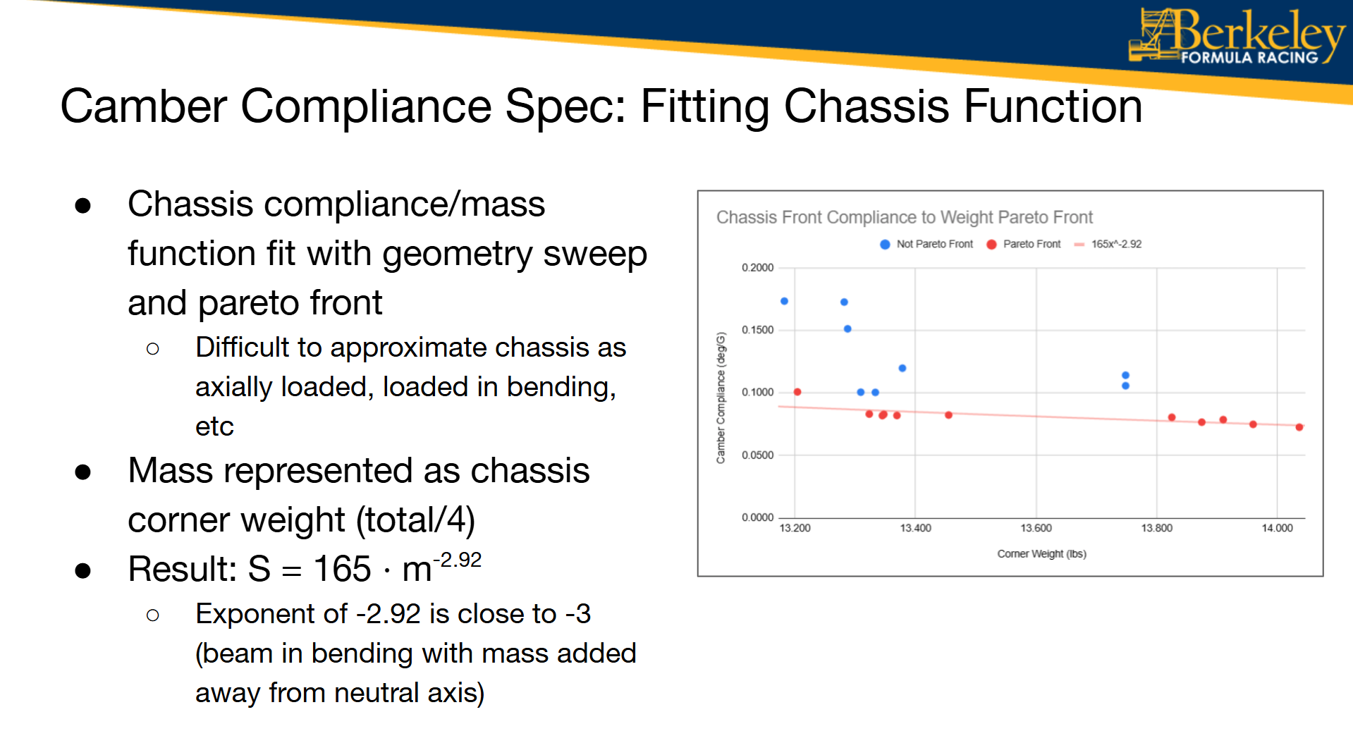
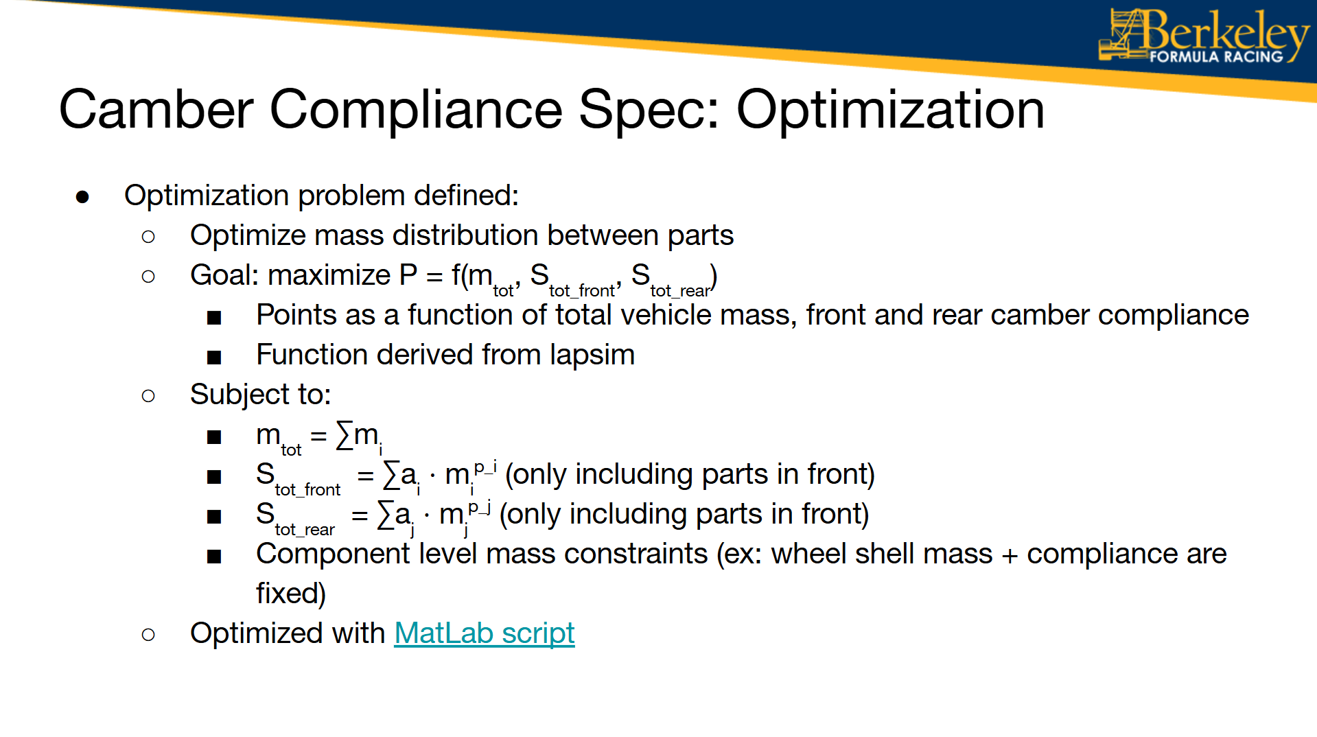
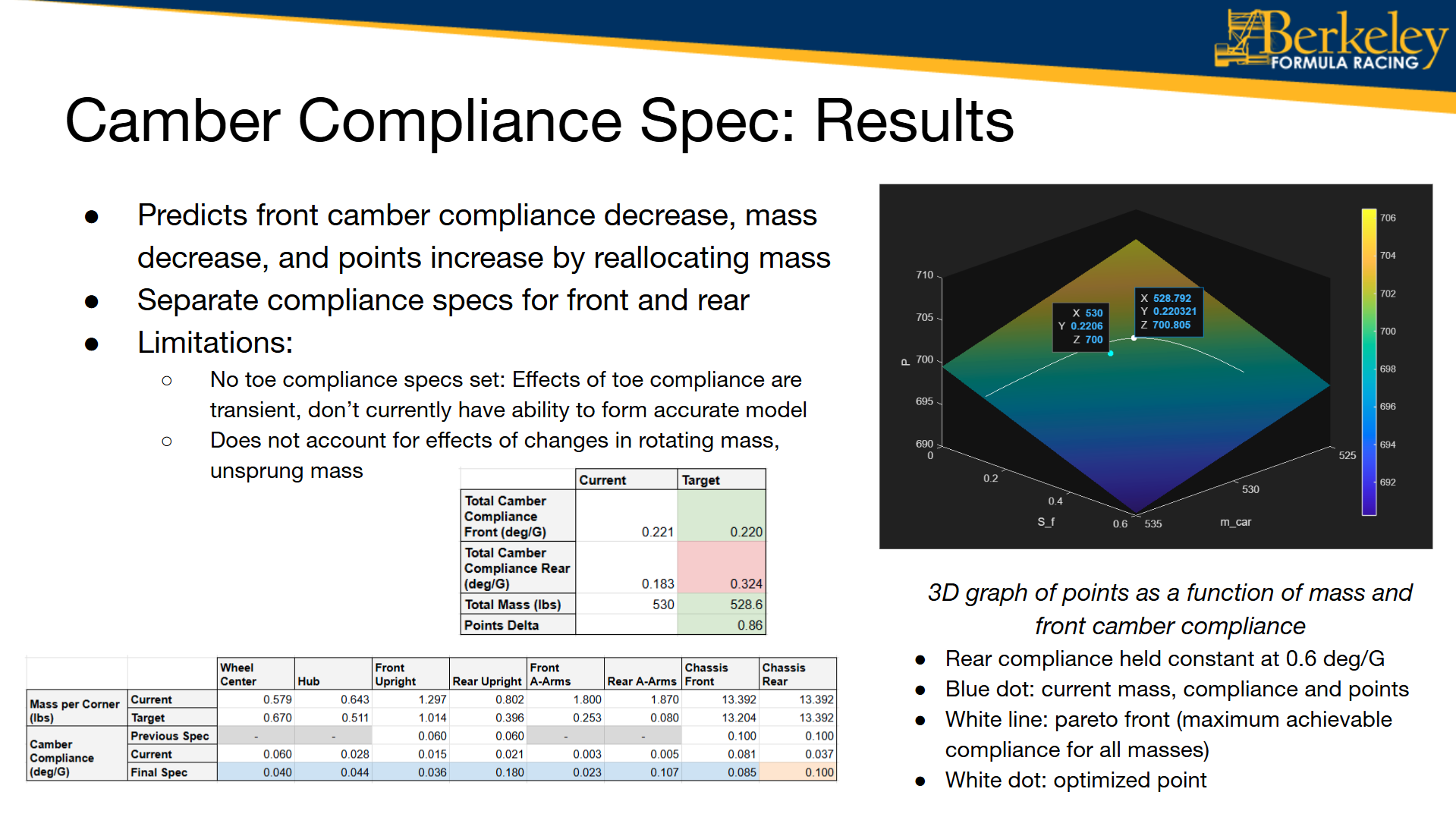
This project involved the creation of a model to set systems level compliance specifications for our B26 FSAE car, and optimize the distribute of camber compliance design specifications between all parts that are structurally loaded under cornering.
MATLAB Code
clear; close; clc; clf
%%%%%%%%%%%%%%% FSAE COMPLIANCE SOLVER %%%%%%%%%%%%%%%
% V1.0
% 10/22/2025
% INPUTS
% Wheel Wheel Hub Front Rear Front Rear Chassis Chassis
% Shell Center Upright Upright A-Arms A-Arms Front Rear
S_i = [ 0.033 0.060 0.028 0.0174 0.021 0.0033 0.0046 0.0813 0.0367 ]; % Initial camber compliance in deg/G
% 0.015 % Old number from Aaron's spreadsheet
m_i = [ 4.197 0.579 0.643 1.297 0.802 1.80 1.87 13.392 13.392 ]; % Initial mass in lbs
m_min = [ 4.197 0 0.643 0 0.5 1.80 1.87 13.204 13.392 ]; % Mass lower bound for optimization in lbs
%m_min = [ 4.197 0 0.643 0 0.5 1.80 1.87 13.204 13.392 ]; % Realistic m_min bounds representing achievable changes
p = [ 2 3 2 3 3 1 1 2.92 2.92 ]; % Exponent for compliance to mass equation, S = a*m^-p % 2.92
n = [ 4 4 4 2 2 2 2 2 2 ]; % number of each part on the car
N = numel(n);
parts = [ "Wheel Shell", "Wheel Center", "Hub", "Front Upright", "Rear Upright", "Front A-Arms", "Rear A-Arms", "Chassis Front", "Chassis Rear" ];
idx_Sf = [1 1 1 1 0 1 0 1 0]; % Index of which parts are included in front compliance
idx_Sr = [1 1 1 0 1 0 1 0 1]; % Index of which parts are included in rear compliance
a = S_i .* m_i .^ p
m_toti = sum(m_i .* n);
m_cari = 530;
m_base = m_cari - m_toti;
S_fi = sum(S_i .* idx_Sf);
S_ri = sum(S_i .* idx_Sr);
P_i = obj(m_i, p, a, m_base, m_cari, S_fi, S_ri, n);
% OPTIMIZATION
lb = 1e-9 * ones(size(m_i));
ub = [];
lb(m_min ~= 0) = m_min(m_min ~= 0);
Aeq = n;
M = fmincon( @(m) -obj( m, p, a, m_base, m_cari, S_fi, S_ri, n ), m_i, [], [], [], [], lb, ub );
S = a .* 1 ./ (M .^ p);
M_tot = sum(n .* M);
m_carf = m_base + M_tot;
S_f = sum(S .* idx_Sf);
S_r = sum(S .* idx_Sr);
P_f = obj( M, p, a, m_base, m_cari, S_fi, S_ri, n );
m_range = 527:0.25:535;
T = zeros(numel(m_range), N + 4);
index = 1;
for i = m_range
beq = i - m_base;
T(index, 1:N) = fmincon( @(m) -obj( m, p, a, m_base, m_cari, S_fi, S_ri, n ), m_i, [], [], Aeq, beq, lb, ub );
T(index, N+1) = m_base + sum(T(index, 1:N).*n);
T(index, N+2) = sum( a .* 1 ./ (T(index, 1:N) .^ p) .* idx_Sf );
T(index, N+3) = sum( a .* 1 ./ (T(index, 1:N) .^ p) .* idx_Sr );
T(index, N+4) = obj( T(index, 1:N), p, a, m_base, m_cari, S_fi, S_ri, n );
index = index + 1;
end
% GRAPH
m_carRange = linspace(525,535,150); %linspace(527,550,150);
S_fRange = linspace(0,0.6,150); %linspace(0,1,150);
S_rRange = 0.6;
% Grid
[M_p1, SF] = meshgrid(m_carRange, S_fRange);
P = 700 + (-0.7*(M_p1-530)) + (((SF-S_fi)/0.1)*(-1.47) + ((S_rRange-S_ri)/0.1)*(-0.1) - 1.548*((SF-S_fi)*(S_rRange-S_ri)));
% 3D colored surface
hold on
surf(M_p1, SF, P); shading interp
alpha(0.5)
xlabel('m\_car'); ylabel('S\_f'); zlabel('P'); colorbar
view(135,30)
plot3(m_range, T(:, N+2), T(:, N+4), 'Color', 'w') % Plot frontier line
plot3(m_cari, S_fi, 700, 'o', 'Color', 'c', 'MarkerSize', 5, 'MarkerFaceColor','c') % Plot initial point
plot3(m_carf, S_f, P_f, 'o', 'Color', 'w', 'MarkerSize', 5, 'MarkerFaceColor','w') % Plot most optimal point
zlim([680 720])
% 2D graph
m_partRange = linspace(0,20,10000).';
T_2 = m_partRange .^ -p .* a;
colors = {'r', 'w', 'r', 'g', 'b', 'r', 'r', 'r', 'r'};
figure(2)
hold on
plot(m_partRange, T_2)
xlim([0,5])
ylim([0,1])
%set(gca, 'XScale', 'log')
%set(gca, 'YScale', 'log')
hCurves = gobjects(N,1);
for i = 1:N
hCurves(i) = plot(m_partRange, T_2(:, i), 'DisplayName', parts{i}); %, colors{i}
end
plot(m_i, S_i, 'ko', 'MarkerFaceColor', 'c', 'MarkerSize', 6, 'DisplayName', 'data points');
plot(M, S, 'ko', 'MarkerFaceColor', 'w', 'MarkerSize', 6, 'DisplayName', 'data points');
legend([hCurves]);
% TABLE
T = array2table([[S_i S_fi S_ri]; [S S_f S_r]; [m_i m_cari 0]; [M m_carf 0]], ...
'RowNames', {'S_initial (deg/G)','S_opt (deg/G)','m_initial (lbs)','m_opt (lbs)' }, ...
'VariableNames', [parts "Total (Front)" "Total (Rear)"]);
disp(T);
disp([P_i P_f]);
% FUNCTIONS
function P_opt = obj(m, p, a, m_base, m_cari, S_fi, S_ri, n)
m_car = m_base + sum(n .* m);
S_all = a .* 1 ./ (m .^ p);
idx_Sf = [1 1 1 1 0 1 0 1 0];
S_f = sum(S_all .* idx_Sf);
idx_Sr = [1 1 1 0 1 0 1 0 1];
S_r = sum(S_all .* idx_Sr);
m_delta = m_car - m_cari;
S_fdelta = S_f - S_fi;
S_rdelta = S_r - S_ri;
P_opt = 700 + (-0.7*m_delta) + ((S_fdelta/0.1)*(-1.47) + (S_rdelta/0.1)*(-0.1) - 1.548*(S_fdelta*S_rdelta));
end